Dynamic ranges in Excel: when to use OFFSET or a table
Keep totals and drop-down choices in sync as rows are added. See how OFFSET and COUNTA work, what happens when an ID is blank, and how to use Excel tables instead.
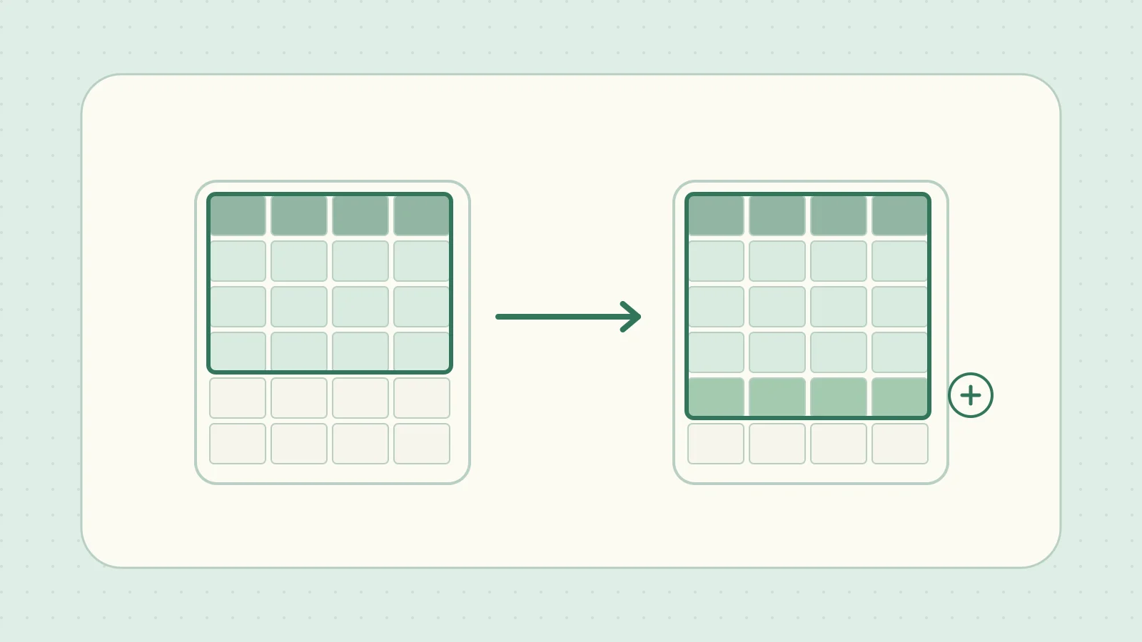
You add a product to an Excel list, but the total and drop-down choices stay the same. If the reference is still A2:A10, the new eleventh row is outside it. A dynamic range lets Excel determine where the list ends, so the person updating it does not have to edit formulas too.
Count rows and columns with OFFSET
For a contiguous list, count the headers and product IDs to supply the height and width to OFFSET. Build this sample on Sheet1 and enter the sum formula on a different sheet. Keep the Japanese header text as shown so the structured references later in the article work.
| Cell | Column A | Column B | Column C |
|---|---|---|---|
| Row 1 | 商品ID (product ID) |
商品名 (product name) |
数量 (quantity) |
| Row 2 | A01 | Pen | 4 |
| Row 3 | A02 | Notebook | 6 |
=SUM(OFFSET(Sheet1!$A$1,0,0,COUNTA(Sheet1!$A$1:$A$1000),COUNTA(Sheet1!$A$1:$Z$1)))
Start at A1 with zero row and column offsets. The count in column A gives the height, and the header count in row 1 gives the width. The example returns A1:C3, three rows by three columns, with a total of 10. Add A03, Ruler, and 2 in row 4, and the range expands to A1:C4 with a total of 12. Product IDs are text, and the counted ranges should contain no unrelated data. Microsoft’s OFFSET reference
Now clear just the ID in A3. Column A has three cells to count: the header in A1 and the IDs in A2 and A4. OFFSET therefore returns the first three rows, A1:C3. It still includes the quantity 6 in row 3 but leaves out the quantity 2 in row 4, so the total returns to 10.
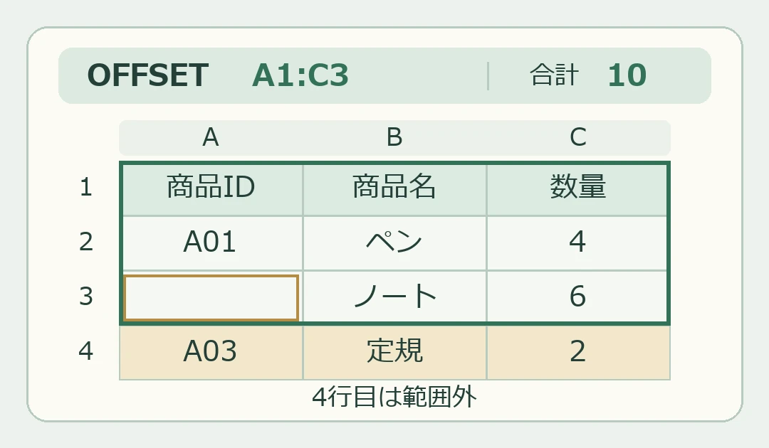
A blank header can similarly cause the last columns to fall outside the range. COUNTA counts cells with formulas returning an empty string (""). In an existing workbook, keep headers and IDs contiguous and check the count limits and blank cells. A missing quantity does not change the height if its ID is present. Microsoft’s COUNTA reference
When headers start in row 2
If row 1 holds a report title, start the list at A2 and count its height and width from row 2 to leave the title out. Moving the sample down one row gives A2:C4 for the header and two products. The total remains 10.
=SUM(OFFSET(Sheet1!$A$2,0,0,COUNTA(Sheet1!$A$2:$A$1000),COUNTA(Sheet1!$A$2:$Z$2)))
Use a table that expands when rows are added
For a new list, select its cells including the headers and choose Insert → Table. Name the table Items. The following formula sums the quantity column from outside the table, and its range expands when you add rows. Microsoft’s guide to structured references
=SUM(Items[数量])
Sum only rows with a product ID
Turn A1:C4 into the Items table and the formula above returns 12 (4 + 6 + 2) even with A3 blank. To include only rows with IDs, use SUMIF with a nonblank condition on the ID column. Here it returns 6 (4 + 2 from rows 2 and 4). Microsoft’s SUMIF reference
=SUMIF(Items[商品ID],"<>",Items[数量])
Keep a drop-down list in sync with the table
For a product-name drop-down on another sheet, go to Formulas → Name Manager in desktop Excel. Create a workbook-scoped name ItemChoices with =Items[商品名] in Refers To. For the input cell, set Data Validation to List and Source to =ItemChoices. The header is excluded and new rows at the end of the table add choices. Fill in names as you add rows so the list has no blank choices. Microsoft’s guide to creating a drop-down list